大模型从0到1｜第八讲：手撕大模型并行训练¶

课程链接：Stanford CS336 Spring 2025 - Lecture 8: Distributed Training Implementation

课程概述¶

上周回顾： 单个 GPU 内的并行化
本周重点： 多 GPU 跨节点的并行化

GPU Node Overview

统一主题： 在两种情况下，计算单元（算术逻辑单元）都远离数据（输入/输出）

核心思想： 编排计算以避免数据传输瓶颈

上周： 通过融合/分块减少内存访问
本周： 通过复制/分片减少跨 GPU/节点的通信

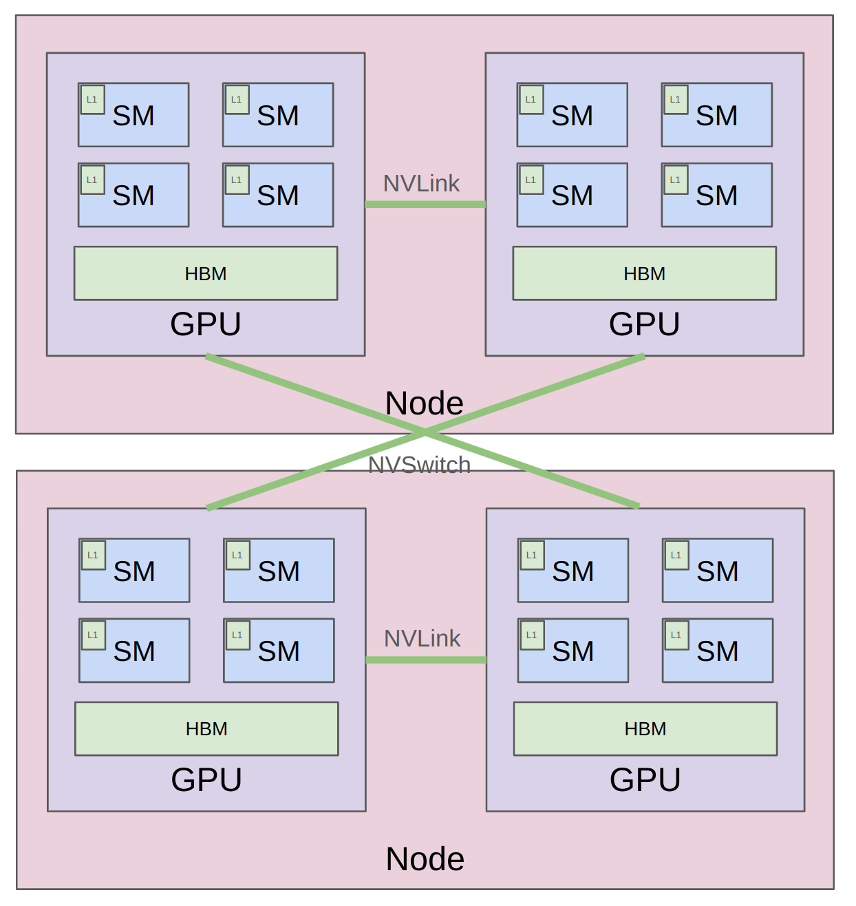
广义的内存层次结构¶

从小/快到大/慢：

单节点，单 GPU： L1 Cache / Shared Memory
单节点，单 GPU： HBM (High Bandwidth Memory)
单节点，多 GPU： NVLink
多节点，多 GPU： NVSwitch

本讲目标： 用代码具体化上一讲的概念

Part 1: 分布式通信/计算的基础模块¶

1.1 集合操作 (Collective Operations)¶

定义： 分布式编程的概念原语

来源： 1980 年代并行编程文献中的经典概念

优势： 比自己管理点对点通信更好/更快的抽象

术语： - World Size（世界大小）： 设备数量（例如 4） - Rank（秩）： 单个设备（例如 0, 1, 2, 3）

1.1.1 Broadcast（广播）¶

Broadcast

操作： 将一个设备的数据复制到所有设备

用途： 分发模型参数、配置信息

1.1.2 Scatter（分散）¶

Scatter

操作： 将数据分割并分发到各个设备

用途： 分发数据批次

1.1.3 Gather（收集）¶

Gather

操作： 从所有设备收集数据到一个设备

用途： 收集预测结果、日志信息

1.1.4 Reduce（归约）¶

Reduce

操作： 对所有设备的数据执行关联/交换操作（sum, min, max）

用途： 计算全局统计量

1.1.5 All-Gather（全收集）¶

All-Gather

操作： 每个设备都收集所有设备的数据

用途： 同步分片数据

1.1.6 Reduce-Scatter（归约分散）¶

Reduce-Scatter

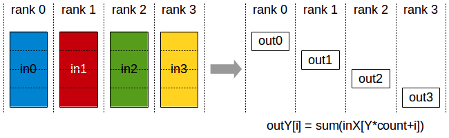
操作： 归约后将结果分散到各设备

用途： 梯度同步的第一步

1.1.7 All-Reduce（全归约）¶

All-Reduce

关键关系： All-Reduce = Reduce-Scatter + All-Gather

用途： 梯度同步（最常用）

记忆技巧¶

Reduce： 执行关联/交换操作（sum, min, max）
Broadcast/Scatter： 是 Gather 的逆操作
All： 目标是所有设备

1.2 硬件架构¶

经典架构（家用）¶

Classic Architecture

同节点 GPU： 通过 PCIe 总线通信（v7.0, 16 lanes => 242 GB/s）
跨节点 GPU： 通过以太网通信（~200 MB/s）

现代架构（数据中心）¶

Modern Architecture

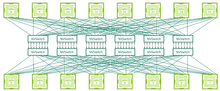
节点内： NVLink 直连 GPU，绕过 CPU
跨节点： NVSwitch 直连 GPU，绕过以太网

H100 规格： - 18 个 NVLink 4.0 链路 - 总带宽：900 GB/s - 对比 HBM 带宽：3.9 TB/s

查看硬件拓扑：

nvidia-smi topo -m

1.3 NVIDIA Collective Communication Library (NCCL)¶

功能： 将集合操作转换为 GPU 间传输的底层数据包

工作流程： 1. 检测硬件拓扑（节点数、交换机、NVLink/PCIe） 2. 优化 GPU 间路径 3. 启动 CUDA kernel 发送/接收数据

参考： NCCL Talk

1.4 PyTorch Distributed (`torch.distributed`)¶

文档： PyTorch Distributed

功能： - 提供集合操作的简洁接口（如 all_gather_into_tensor） - 支持多种后端：gloo (CPU), nccl (GPU) - 支持高级算法（如 FullyShardedDataParallel）

示例代码：All-Reduce¶

def collective_operations_main(rank: int, world_size: int):
    setup(rank, world_size)

    # 创建张量
    tensor = torch.tensor([0., 1, 2, 3], device=get_device(rank)) + rank

    print(f"Rank {rank} [before all-reduce]: {tensor}")

    # 执行 all-reduce（原地修改）
    dist.all_reduce(tensor=tensor, op=dist.ReduceOp.SUM, async_op=False)

    print(f"Rank {rank} [after all-reduce]: {tensor}")

    cleanup()

输出示例（world_size=4）：

Rank 0 [before]: [0., 1., 2., 3.]
Rank 1 [before]: [1., 2., 3., 4.]
Rank 2 [before]: [2., 3., 4., 5.]
Rank 3 [before]: [3., 4., 5., 6.]

Rank 0 [after]: [6., 10., 14., 18.]  # 每个位置求和
Rank 1 [after]: [6., 10., 14., 18.]
Rank 2 [after]: [6., 10., 14., 18.]
Rank 3 [after]: [6., 10., 14., 18.]

示例代码：Reduce-Scatter + All-Gather¶

# Reduce-Scatter
input = torch.arange(world_size, dtype=torch.float32, device=get_device(rank)) + rank
output = torch.empty(1, device=get_device(rank))

print(f"Rank {rank} [before reduce-scatter]: input = {input}, output = {output}")
dist.reduce_scatter_tensor(output=output, input=input, op=dist.ReduceOp.SUM, async_op=False)
print(f"Rank {rank} [after reduce-scatter]: input = {input}, output = {output}")

# All-Gather
input = output
output = torch.empty(world_size, device=get_device(rank))

print(f"Rank {rank} [before all-gather]: input = {input}, output = {output}")
dist.all_gather_into_tensor(output_tensor=output, input_tensor=input, async_op=False)
print(f"Rank {rank} [after all-gather]: input = {input}, output = {output}")

验证： All-Reduce = Reduce-Scatter + All-Gather ✅

1.5 性能测试¶

All-Reduce 性能测试¶

def all_reduce(rank: int, world_size: int, num_elements: int):
    setup(rank, world_size)

    # 创建张量
    tensor = torch.randn(num_elements, device=get_device(rank))

    # Warmup
    dist.all_reduce(tensor=tensor, op=dist.ReduceOp.SUM, async_op=False)
    torch.cuda.synchronize()
    dist.barrier()

    # 计时
    start_time = time.time()
    dist.all_reduce(tensor=tensor, op=dist.ReduceOp.SUM, async_op=False)
    torch.cuda.synchronize()
    dist.barrier()
    end_time = time.time()

    duration = end_time - start_time

    # 计算有效带宽
    size_bytes = tensor.element_size() * tensor.numel()
    sent_bytes = size_bytes * 2 * (world_size - 1)  # 2x：发送输入 + 接收输出
    total_duration = world_size * duration
    bandwidth = sent_bytes / total_duration

    print(f"Rank {rank}: bandwidth = {round(bandwidth / 1024**3)} GB/s")

    cleanup()

测试：

spawn(all_reduce, world_size=4, num_elements=100 * 1024**2)

Part 2: 分布式训练策略¶

示例模型： 深度 MLP（多层感知机）

原因： MLP 是 Transformer 的计算瓶颈，具有代表性

三种并行策略： 1. Data Parallelism（数据并行）： 沿批次维度切分 2. Tensor Parallelism（张量并行）： 沿宽度维度切分 3. Pipeline Parallelism（流水线并行）： 沿深度维度切分

2.1 Data Parallelism（数据并行）¶

Data Parallelism

分片策略： 每个 rank 获得数据的一个切片

实现代码¶

def data_parallelism_main(rank: int, world_size: int, data: torch.Tensor, num_layers: int, num_steps: int):
    setup(rank, world_size)

    # 获取此 rank 的数据切片
    batch_size = data.size(0)
    local_batch_size = batch_size // world_size
    start_index = rank * local_batch_size
    end_index = start_index + local_batch_size
    data = data[start_index:end_index].to(get_device(rank))

    # 创建模型参数（每个 rank 拥有所有参数）
    params = [get_init_params(num_dim, num_dim, rank) for i in range(num_layers)]
    optimizer = torch.optim.AdamW(params, lr=1e-3)

    for step in range(num_steps):
        # 前向传播
        x = data
        for param in params:
            x = x @ param
            x = F.gelu(x)
        loss = x.square().mean()

        # 反向传播
        loss.backward()

        # 同步梯度（与标准训练的唯一区别）
        for param in params:
            dist.all_reduce(tensor=param.grad, op=dist.ReduceOp.AVG, async_op=False)

        # 更新参数
        optimizer.step()

        print(f"Rank {rank}: step = {step}, loss = {loss.item()}")

    cleanup()

关键观察¶

不同之处： - ✅ 每个 rank 的 Loss 不同（基于本地数据计算） - ✅ 梯度通过 all-reduce 同步，所有 rank 相同 - ✅ 因此，参数在所有 rank 上保持一致

通信成本： - 每步需要 all-reduce 所有梯度 - 通信量 = 模型参数量

优点： - 实现简单 - 扩展性好（理想情况下线性加速）

缺点： - 每个 GPU 需要存储完整模型 - 通信开销随模型大小增长

2.2 Tensor Parallelism（张量并行）¶

Tensor Parallelism

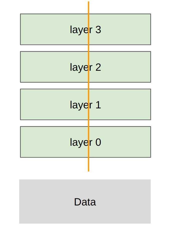
分片策略： 每个 rank 获得每层的一部分，传输所有数据/激活

实现代码¶

def tensor_parallelism_main(rank: int, world_size: int, data: torch.Tensor, num_layers: int):
    setup(rank, world_size)

    data = data.to(get_device(rank))
    batch_size = data.size(0)
    num_dim = data.size(1)
    local_num_dim = num_dim // world_size  # 分片 num_dim

    # 创建模型（每个 rank 获得 1/world_size 的参数）
    params = [get_init_params(num_dim, local_num_dim, rank) for i in range(num_layers)]

    # 前向传播
    x = data
    for i in range(num_layers):
        # 计算激活（batch_size x local_num_dim）
        x = x @ params[i]  # 注意：这只是参数的一个切片
        x = F.gelu(x)

        # 为激活分配内存（world_size x batch_size x local_num_dim）
        activations = [torch.empty(batch_size, local_num_dim, device=get_device(rank)) 
                      for _ in range(world_size)]

        # 通过 all-gather 发送激活
        dist.all_gather(tensor_list=activations, tensor=x, async_op=False)

        # 拼接得到 batch_size x num_dim
        x = torch.cat(activations, dim=1)

    print(f"Rank {rank}: forward pass produced activations {summarize_tensor(x)}")

    # 反向传播：作业练习

    cleanup()

关键观察¶

内存分布： - ✅ 每个 rank 只存储部分参数 - ✅ 激活需要在所有 rank 间通信

通信成本： - 每层需要 all-gather 激活 - 通信量 = 激活大小 × 层数

优点： - 可以训练更大的模型（参数分片） - 适合宽模型

缺点： - 通信频繁（每层都需要通信） - 实现复杂度高

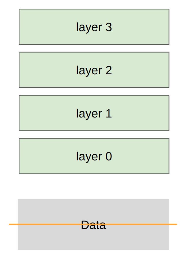
2.3 Pipeline Parallelism（流水线并行）¶

Pipeline Parallelism

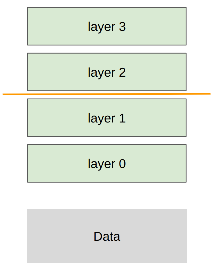
分片策略： 每个 rank 获得层的子集，传输所有数据/激活

实现代码¶

def pipeline_parallelism_main(rank: int, world_size: int, data: torch.Tensor, 
                             num_layers: int, num_micro_batches: int):
    setup(rank, world_size)

    data = data.to(get_device(rank))
    batch_size = data.size(0)
    num_dim = data.size(1)

    # 分割层
    local_num_layers = num_layers // world_size

    # 每个 rank 获得层的子集
    local_params = [get_init_params(num_dim, num_dim, rank) for i in range(local_num_layers)]

    # 前向传播

    # 分成 micro-batch 以最小化气泡
    micro_batch_size = batch_size // num_micro_batches
    if rank == 0:
        micro_batches = data.chunk(chunks=num_micro_batches, dim=0)
    else:
        micro_batches = [torch.empty(micro_batch_size, num_dim, device=get_device(rank)) 
                        for _ in range(num_micro_batches)]

    for x in micro_batches:
        # 从前一个 rank 接收激活
        if rank - 1 >= 0:
            dist.recv(tensor=x, src=rank - 1)

        # 计算分配给此 rank 的层
        for param in local_params:
            x = x @ param
            x = F.gelu(x)

        # 发送到下一个 rank
        if rank + 1 < world_size:
            print(f"Rank {rank}: sending {summarize_tensor(x)} to rank {rank + 1}")
            dist.send(tensor=x, dst=rank + 1)

    # 未处理：重叠通信/计算以消除流水线气泡

    # 反向传播：作业练习

    cleanup()

关键观察¶

Micro-Batch 技术： - 将批次分成更小的 micro-batch - 减少流水线气泡（idle time） - 提高 GPU 利用率

通信模式： - 点对点通信（send/recv） - 只在相邻 rank 间通信

优点： - 内存效率高（每个 GPU 只存储部分层） - 适合深模型

缺点： - 流水线气泡导致 GPU 空闲 - 需要精心设计 micro-batch 调度

并行策略对比¶

策略	分片维度	通信模式	内存效率	适用场景
Data Parallelism	Batch	All-Reduce	低（完整模型）	小模型，大批次
Tensor Parallelism	Width	All-Gather	中（参数分片）	宽模型
Pipeline Parallelism	Depth	Send/Recv	高（层分片）	深模型

混合并行策略¶

实际应用： 通常组合多种策略

示例：GPT-3 训练 - Data Parallelism: 跨节点 - Tensor Parallelism: 节点内（利用 NVLink） - Pipeline Parallelism: 跨层

其他并行维度： - Sequence Parallelism： 沿序列长度切分 - Expert Parallelism： MoE 模型中的专家并行

高级话题¶

通信与计算重叠¶

目标： 在计算时进行通信，隐藏通信延迟

技术： - 异步通信（async_op=True） - 梯度累积 - 流水线调度

内存优化¶

权衡： - 重计算（Recomputation）： 节省内存，增加计算 - 存储（Memory）： 增加内存，减少计算 - 通信（Communication）： 存储在其他 GPU，需要通信

ZeRO 优化： - ZeRO-1: 优化器状态分片 - ZeRO-2: 梯度分片 - ZeRO-3: 参数分片

课程未涵盖的内容¶

更复杂的模型： - Attention 机制 - 更复杂的架构

更多优化： - 通信/计算重叠 - 更复杂的调度

其他框架： - JAX/TPU： 只需定义模型和分片策略，编译器处理其余部分 - 参考：Levanter - PyTorch： 本课程使用，可以看到如何从原语构建

总结¶

核心概念¶

多种并行化方式：
Data（batch）
Tensor/Expert（width）
Pipeline（depth）
Sequence（length）
三种权衡：
重计算（Recompute）
存储在内存（Memory）
存储在其他 GPU 并通信（Communicate）
硬件趋势：
硬件越来越快
但总是想要更大的模型
因此总会有这种层次结构

关键原则¶

统一主题： 编排计算以避免数据传输瓶颈

上周： 单 GPU 内 - 减少内存访问（融合/分块）
本周： 多 GPU 间 - 减少通信（复制/分片）

实践建议¶

Setup 函数¶

def setup(rank: int, world_size: int):
    # 指定 master 位置（rank 0），用于协调
    os.environ["MASTER_ADDR"] = "localhost"
    os.environ["MASTER_PORT"] = "15623"

    if torch.cuda.is_available():
        dist.init_process_group("nccl", rank=rank, world_size=world_size)
    else:
        dist.init_process_group("gloo", rank=rank, world_size=world_size)

def cleanup():
    torch.distributed.destroy_process_group()

多进程启动¶

from lecture_08_utils import spawn

# 启动 4 个进程
spawn(your_function, world_size=4, **kwargs)

延伸阅读¶

NCCL 性能： - How to reason about operations - Sample benchmark code

分布式训练： - PyTorch Distributed Tutorial - FSDP Documentation - DeepSpeed - Megatron-LM

硬件： - NVLink Documentation - H100 Datasheet

作业练习¶

实现 Tensor Parallelism 的反向传播
实现 Pipeline Parallelism 的反向传播
测量不同并行策略的通信开销
实现混合并行策略（Data + Tensor）
优化流水线调度以减少气泡

大模型从0到1｜第八讲：手撕大模型并行训练¶

课程概述¶

广义的内存层次结构¶

Part 1: 分布式通信/计算的基础模块¶

1.1 集合操作 (Collective Operations)¶

1.1.1 Broadcast（广播）¶

1.1.2 Scatter（分散）¶

1.1.3 Gather（收集）¶

1.1.4 Reduce（归约）¶

1.1.5 All-Gather（全收集）¶

1.1.6 Reduce-Scatter（归约分散）¶

1.1.7 All-Reduce（全归约）¶

记忆技巧¶

1.2 硬件架构¶

经典架构（家用）¶

现代架构（数据中心）¶

1.3 NVIDIA Collective Communication Library (NCCL)¶

1.4 PyTorch Distributed (torch.distributed)¶

示例代码：All-Reduce¶

示例代码：Reduce-Scatter + All-Gather¶

1.5 性能测试¶

All-Reduce 性能测试¶

Part 2: 分布式训练策略¶

2.1 Data Parallelism（数据并行）¶

实现代码¶

关键观察¶

2.2 Tensor Parallelism（张量并行）¶

实现代码¶

关键观察¶

2.3 Pipeline Parallelism（流水线并行）¶

实现代码¶

关键观察¶

并行策略对比¶

混合并行策略¶

高级话题¶

通信与计算重叠¶

内存优化¶

课程未涵盖的内容¶

总结¶

核心概念¶

关键原则¶

实践建议¶

Setup 函数¶

多进程启动¶

延伸阅读¶

作业练习¶

💬 评论

1.4 PyTorch Distributed (`torch.distributed`)¶