大模型从0到1｜第六讲：手写高性能算子

课程链接：Stanford CS336 Spring 2025 - Lecture 6: Writing Fast Kernels

---

课程概述

上节课回顾： GPU 的高层次概述和性能分析
本节课重点： 性能测试/分析 + 手写 GPU 算子

核心内容：

• Benchmarking 和 Profiling 技术
• Kernel Fusion（算子融合）的动机
• 三种编写算子的方式：CUDA、Triton、PyTorch 编译

---

Part 1: GPU 架构回顾

1.1 硬件架构

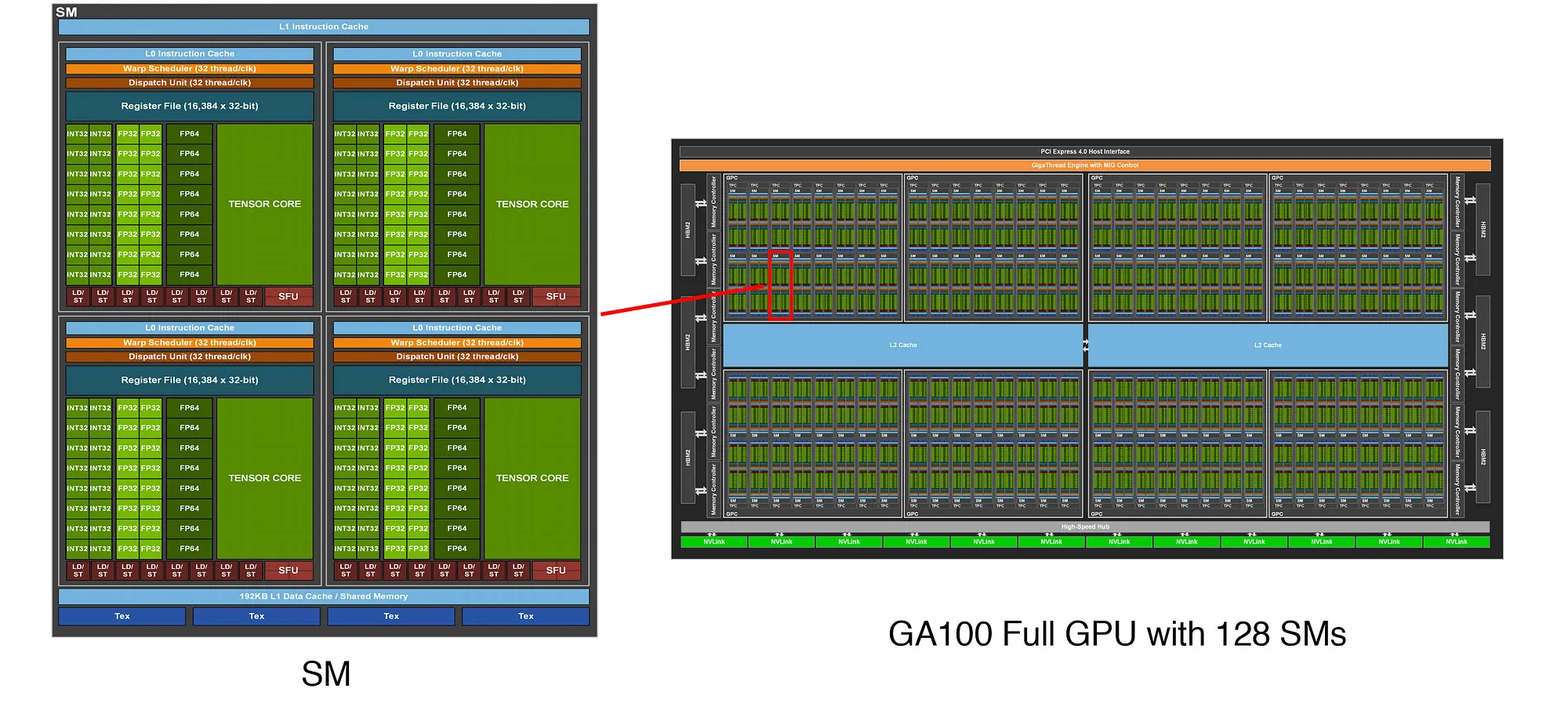
计算单元：

• Streaming Multiprocessors (SMs) [A100: 108个]

内存层次：

• DRAM [A100: 80GB] - 容量大，速度慢
• L2 Cache [A100: 40MB]
• L1 Cache [A100: 192KB per SM] - 容量小，速度快

1.2 执行模型

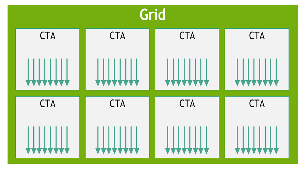
三层结构：

• Thread（线程）： 处理单个索引 i，即执行 f(i)
• Thread Block（线程块）： 调度到单个 SM 上，又称 CTA (Concurrent Thread Arrays)
• Grid（网格）： 线程块的集合

为什么需要 Thread Block？

• 共享内存（Shared Memory）： 线程块内的线程可以共享内存（速度与 L1 Cache 相当）[A100: 164KB]
• 同步机制： 可以在块内同步线程（但不能跨块同步）
• 设计原则： 将读取相似数据的 f(i) 分组到一起

1.3 硬件与执行的交互

Wave Quantization 问题：

• 线程块以”波次”调度到 SM 上
• 最后一波可能线程块较少，导致部分 SM 空闲（低占用率）
• 解决方案： 让线程块数量能被 SM 数量整除
• 经验法则： 线程块数量应 >= 4x SM 数量

挑战： 硬件的某些方面对执行模型是隐藏的（如调度策略、SM 数量）

1.4 算术强度 (Arithmetic Intensity)

定义： 算术强度 = FLOPs 数量 / 字节数

• 高算术强度： 计算密集型（compute-bound）✅ 好
• 低算术强度： 内存密集型（memory-bound）❌ 差

通用规则：

• 矩阵乘法：计算密集型
• 其他大部分操作：内存密集型

---

Part 2: Benchmarking 和 Profiling

2.1 为什么需要性能测试？

重要性： 必须对代码进行 benchmark 和 profile！

虽然可以阅读规格表和论文，但性能取决于：

• 库版本
• 硬件配置
• 工作负载特性

没有替代品： 必须亲自测试你的代码

2.2 示例：MLP 模型

class MLP(nn.Module):
    """简单的 MLP: linear -> GeLU -> linear -> GeLU -> ..."""
    def __init__(self, dim: int, num_layers: int):
        super().__init__()
        self.layers = nn.ModuleList([nn.Linear(dim, dim) for _ in range(num_layers)])

    def forward(self, x: torch.Tensor):
        for layer in self.layers:
            x = layer(x)
            x = torch.nn.functional.gelu(x)
        return x

2.3 Benchmarking：测量时间

目的： 测量操作的实际运行时间

用途：

• 比较不同实现（哪个更快？）
• 理解性能如何扩展（如随维度变化）

实现要点：

def benchmark(description: str, run: Callable, num_warmups: int = 1, num_trials: int = 3):
    # Warmup: 首次运行可能较慢（编译、缓存等）
    for _ in range(num_warmups):
        run()
    torch.cuda.synchronize()  # 等待 CUDA 线程完成（重要！）
    
    # 正式计时
    times = []
    for trial in range(num_trials):
        start_time = time.time()
        run()
        torch.cuda.synchronize()  # 重要！
        end_time = time.time()
        times.append((end_time - start_time) * 1000)
    
    return mean(times)

测试场景：

• 扩展步数（num_steps）
• 扩展层数（num_layers）
• 扩展批大小（batch_size）
• 扩展维度（dim）

注意： 由于 CUDA kernel 的非均质性、硬件等因素，时间并不总是可预测的

2.4 Profiling：分析瓶颈

目的： 了解时间花在哪里

深层价值： 帮助理解底层调用了什么

PyTorch Profiler：

def profile(description: str, run: Callable, with_stack: bool = False):
    # Warmup
    for _ in range(num_warmups):
        run()
    torch.cuda.synchronize()
    
    # 使用 profiler 运行
    with torch.profiler.profile(
            activities=[ProfilerActivity.CPU, ProfilerActivity.CUDA],
            with_stack=with_stack) as prof:
        run()
        torch.cuda.synchronize()
    
    # 打印表格
    table = prof.key_averages().table(sort_by="cuda_time_total",
                                      max_name_column_width=80,
                                      row_limit=10)
    return table

观察结果：

• 可以看到实际调用的 CUDA kernel
• 不同的 tensor 维度会调用不同的 CUDA kernel
• Kernel 名称透露实现信息
  • 例如：cutlass_80_simt_sgemm_256x128_8x4_nn_align1
  • cutlass: NVIDIA 的线性代数 CUDA 库
  • 256x128: tile 大小

Flame Graph： 可视化堆栈跟踪，显示时间分布

---

Part 3: Kernel Fusion 动机

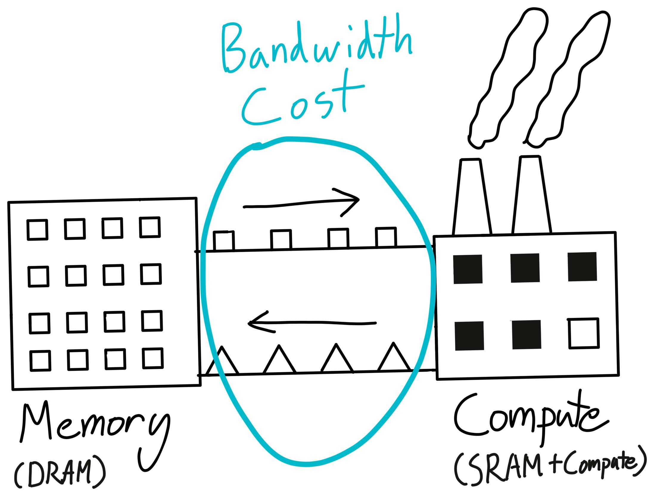
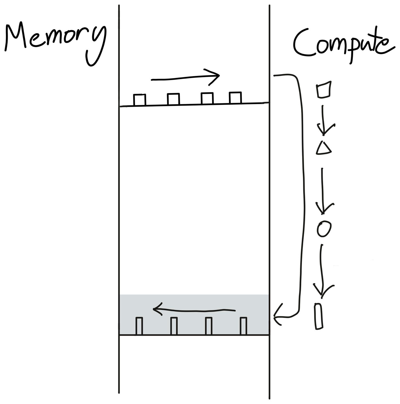
3.1 仓库与工厂的类比

参考： Horace He’s Blog Post

类比：

• 仓库 ≈ DRAM (HBM)
• 工厂 ≈ SRAM (L1 Cache / Shared Memory)

深入理解这个类比

现实世界的工厂运作：

想象你经营一家制造工厂：

• 仓库（Warehouse）： 远离工厂，容量巨大，但运输慢且昂贵
• 工厂车间（Factory Floor）： 空间有限，但工人可以快速拿取材料并加工

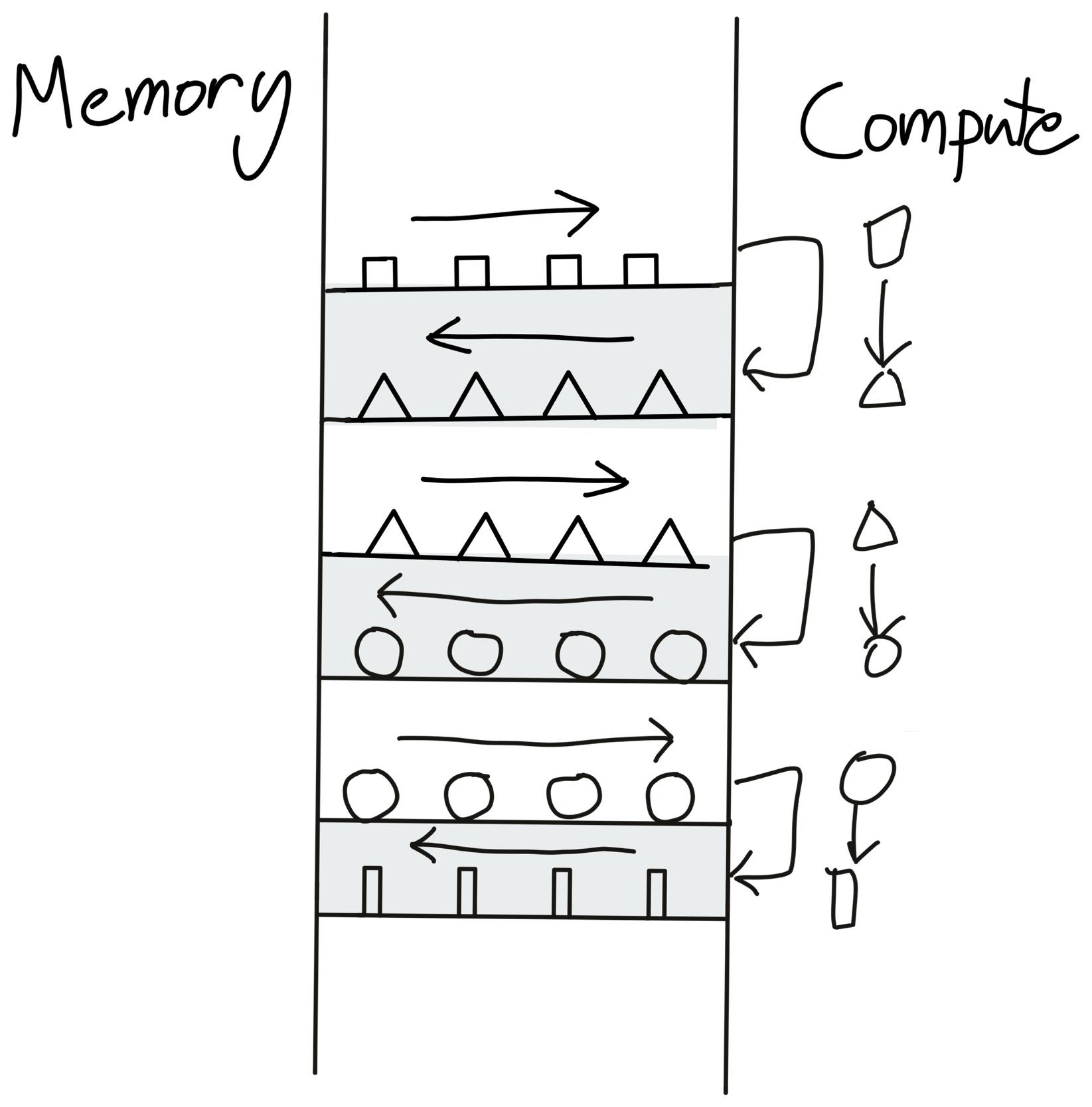
最优策略：

1. 一次性从仓库运来一批原材料
2. 在工厂车间内完成所有加工步骤
3. 一次性把成品运回仓库

最差策略：

1. 从仓库拿原材料 → 加工一步 → 送回仓库
2. 再从仓库拿 → 加工第二步 → 送回仓库
3. 重复多次…

每次往返仓库都是巨大的时间浪费！

---

映射到 GPU 内存：

现实世界	GPU 硬件	特性
仓库	DRAM/HBM	容量大（40-80GB），带宽低（~2 TB/s）
运输卡车	内存总线	带宽有限，往返成本高
工厂车间	SRAM (L1/Shared Memory)	容量小（192KB），带宽高（19 TB/s）
工人	计算单元 (CUDA Cores)	执行实际计算

关键数字对比（A100 GPU）：

• DRAM 带宽： ~2 TB/s（慢 10 倍）
• SRAM 带宽： ~19 TB/s（快 10 倍）
• 容量差异： DRAM 是 SRAM 的 ~400,000 倍

---

未融合操作的问题

场景： 计算 output = gelu(x + bias)

未融合的执行流程：

步骤 1: x + bias
  DRAM → SRAM: 读取 x (慢)
  DRAM → SRAM: 读取 bias (慢)
  SRAM 计算: x + bias (快)
  SRAM → DRAM: 写入 temp (慢)
  
步骤 2: gelu(temp)
  DRAM → SRAM: 读取 temp (慢！刚写进去又读出来)
  SRAM 计算: gelu(temp) (快)
  SRAM → DRAM: 写入 output (慢)

内存访问次数：

• 读取：3 次（x, bias, temp）
• 写入：2 次（temp, output）
• 总计：5 次 DRAM 访问 🐌

类比： 就像从仓库拿材料 → 加工一步 → 送回仓库 → 再拿出来 → 加工第二步 → 送回仓库

---

融合操作的优势

融合后的执行流程：

步骤 1+2: fused_gelu_bias(x, bias)
  DRAM → SRAM: 读取 x (慢)
  DRAM → SRAM: 读取 bias (慢)
  SRAM 计算: temp = x + bias (快)
  SRAM 计算: output = gelu(temp) (快，temp 还在 SRAM 中！)
  SRAM → DRAM: 写入 output (慢)

内存访问次数：

• 读取：2 次（x, bias）
• 写入：1 次（output）
• 总计：3 次 DRAM 访问 ⚡

性能提升： 5 → 3，减少了 40% 的内存访问！

类比： 一次性从仓库拿所有材料 → 在工厂内完成所有加工 → 一次性送回成品

---

为什么内存访问是瓶颈？

计算速度 vs 内存速度的差距：

假设处理 1M 个元素（4MB 数据）：

计算时间（在 SRAM 中）：

• 加法：~0.001 ms
• GeLU：~0.01 ms
• 总计：可以忽略不计

内存传输时间（DRAM ↔ SRAM）：

• 未融合：5 次 × 4MB ÷ 2TB/s = 0.01 ms
• 融合：3 次 × 4MB ÷ 2TB/s = 0.006 ms

结论： 内存传输时间 >> 计算时间！

这就是为什么说大多数操作是 memory-bound（内存受限） 而不是 compute-bound（计算受限）。

---

实际性能数据

GeLU 性能对比（dim=16384）：

manual_gelu (未融合):    ~2.5 ms
pytorch_gelu (融合):     ~0.3 ms
cuda_gelu (手写融合):    ~0.5 ms
triton_gelu (融合):      ~0.35 ms

融合带来 5-8 倍性能提升！

---

扩展到更复杂的场景

Transformer 中的典型操作链：

# 未融合（灾难）
x = layer_norm(x)      # DRAM 读写
x = x + residual       # DRAM 读写
x = dropout(x)         # DRAM 读写
x = gelu(x)           # DRAM 读写
# 总计：8 次 DRAM 访问

# 融合（高效）
x = fused_ln_residual_dropout_gelu(x, residual)
# 总计：2 次 DRAM 访问（读 x 和 residual，写 output）

性能提升： 可达 4-10 倍！

---

关键洞察总结

1. DRAM 是瓶颈： 不是计算慢，是数据搬运慢
2. SRAM 是宝贵资源： 容量小但速度快，要充分利用
3. 最小化往返次数： 每次 DRAM 访问都是昂贵的
4. 在 SRAM 中完成尽可能多的工作： 这就是 kernel fusion 的本质

记住： GPU 编程的核心不是”让计算更快”，而是”让数据搬运更少”！

这就是为什么 FlashAttention、Fused LayerNorm 等优化如此重要——它们都在减少内存往返次数。

3.2 未融合 vs 融合

未融合操作： 每个操作都需要 读取 → 计算 → 写入

融合操作： 只需要读写一次

3.3 案例：GeLU 激活函数

GeLU 公式：

gelu(x) = 0.5 * x * (1 + tanh(sqrt(2/π) * (x + 0.044715 * x³)))

两种实现方式：

1. Manual GeLU（未融合）：

   def manual_gelu(x):
       return 0.5 * x * (1 + torch.tanh(
           torch.sqrt(torch.tensor(2.0 / torch.pi)) * 
           (x + 0.044715 * torch.pow(x, 3))
       ))

2. PyTorch GeLU（融合）：

   def pytorch_gelu(x):
       return torch.nn.functional.gelu(x)

性能对比：

• 融合版本显著更快
• Manual 版本调用多个 kernel
• PyTorch 版本只调用一个 kernel

关键洞察： 记住仓库/工厂的类比！

---

Part 4: CUDA Kernels

4.1 CUDA 基础

CUDA 是什么？

• C/C++ 的扩展，带有管理 GPU 的 API
• 简化模型：编写 f(i)，CUDA kernel 为所有 i 计算 f(i)

编程模型：

• Grid: 线程块集合，如 numBlocks = (2, 4), blockDim = (1, 8)
• Thread Block: 线程集合，如 blockIdx = (0, 1)
• Thread: 单个操作单元，如 threadIdx = (0, 3)

编程方式：

• 编写单个线程执行的代码
• 使用 (blockIdx, blockDim, threadIdx) 确定要做什么

4.2 CUDA GeLU 实现

CUDA 代码示例（gelu.cu）：

#include <torch/extension.h>
#include <cuda_runtime.h>

__global__ void gelu_kernel(const float* x, float* y, int n) {
    int idx = blockIdx.x * blockDim.x + threadIdx.x;
    if (idx < n) {
        float val = x[idx];
        float a = 0.79788456f * (val + 0.044715f * val * val * val);
        float exp_2a = expf(2.0f * a);
        float tanh_a = (exp_2a - 1.0f) / (exp_2a + 1.0f);
        y[idx] = 0.5f * val * (1.0f + tanh_a);
    }
}

torch::Tensor gelu(torch::Tensor x) {
    auto y = torch::empty_like(x);
    int n = x.numel();
    int threads = 256;
    int blocks = (n + threads - 1) / threads;
    
    gelu_kernel<<<blocks, threads>>>(
        x.data_ptr<float>(),
        y.data_ptr<float>(),
        n
    );
    
    return y;
}

编译和使用：

from torch.utils.cpp_extension import load_inline

module = load_inline(
    cuda_sources=[cuda_gelu_src],
    cpp_sources=[cpp_gelu_src],
    functions=["gelu"],
    extra_cflags=["-O2"],
    name="inline_gelu",
    build_directory="var/cuda_gelu",
)

cuda_gelu = module.gelu

性能：

• CUDA 实现比 manual 快
• 但不如 PyTorch 实现

局限性：

• 逐元素操作在 CUDA 中容易实现
• 但大多数有趣的操作（matmul、softmax、RMSNorm）需要读取多个值
• 需要考虑共享内存管理等

---

Part 5: Triton Kernels

5.1 Triton 简介

开发者： OpenAI (2021)
目标： 让 GPU 编程更易用

优势：

• 用 Python 编写
• 思考线程块而非单个线程

Triton vs CUDA：

                                    CUDA      Triton
内存合并（从 DRAM 传输）             手动      自动
共享内存管理                         手动      自动
SM 内调度                           手动      自动
跨 SM 调度                          手动      手动

关键点： 编译器做更多工作，实际上可以超越 PyTorch 实现！

5.2 Triton GeLU 实现

@triton.jit
def triton_gelu_kernel(x_ptr, y_ptr, num_elements, BLOCK_SIZE: tl.constexpr):
    # 输入在 x_ptr，输出在 y_ptr
    # |    Block 0    |    Block 1    |  ...  |
    #            BLOCK_SIZE              num_elements
    
    pid = tl.program_id(axis=0)
    block_start = pid * BLOCK_SIZE
    
    # 此线程块应操作的索引
    offsets = block_start + tl.arange(0, BLOCK_SIZE)
    
    # 处理边界
    mask = offsets < num_elements
    
    # 读取
    x = tl.load(x_ptr + offsets, mask=mask)
    
    # 计算 gelu (使用 tanh(a) = (exp(2a) - 1) / (exp(2a) + 1))
    a = 0.79788456 * (x + 0.044715 * x * x * x)
    exp = tl.exp(2 * a)
    tanh = (exp - 1) / (exp + 1)
    y = 0.5 * x * (1 + tanh)
    
    # 存储
    tl.store(y_ptr + offsets, y, mask=mask)

def triton_gelu(x: torch.Tensor):
    y = torch.empty_like(x)
    num_elements = x.numel()
    block_size = 1024
    num_blocks = triton.cdiv(num_elements, block_size)
    
    triton_gelu_kernel[(num_blocks,)](x, y, num_elements, BLOCK_SIZE=block_size)
    return y

调试优势： 可以单步调试 Python 代码！

5.3 PTX 汇编

PTX (Parallel Thread Execution)： GPU 的类汇编语言

可以查看 Triton 生成的 PTX 代码：

• ld.global.* 和 st.global.*：从全局内存读写
• %ctaid.x：块索引，%tid.x：线程索引
• %f*：浮点寄存器，%r*：整数寄存器
• Thread Coarsening： 一个线程同时处理 8 个元素

性能对比：

• Triton 实现几乎与 PyTorch 一样好
• 实际上比我们的朴素 CUDA 实现慢
• 但都远快于 manual 实现

原因：

• Triton 操作块，CUDA 操作线程
• 块允许 Triton 编译器进行其他优化（如线程粗化）

---

Part 6: PyTorch 编译

6.1 torch.compile

第五种方式： 用 Python 编写，编译成 Triton

compiled_gelu = torch.compile(manual_gelu)

优势：

• 自动融合操作
• 无需手写 CUDA 或 Triton
• 性能接近手写实现

检查正确性：

check_equal(compiled_gelu, manual_gelu)

性能： 与 Triton 手写版本相当

---

Part 7: Softmax 案例研究

7.1 Softmax 操作

定义： 对矩阵的每一行进行归一化

[A1 A2 A3]   =>   [A1/A A2/A A3/A]
[B1 B2 B3]   =>   [B1/B B2/B B3/B]

用途：

• Attention 机制
• 生成概率分布

7.2 Manual Softmax（未融合）

def manual_softmax(x):
    # 数值稳定性：减去最大值
    x_max = x.max(dim=-1, keepdim=True)[0]
    x_shifted = x - x_max
    
    # 计算 exp
    exp_x = torch.exp(x_shifted)
    
    # 归一化
    sum_exp = exp_x.sum(dim=-1, keepdim=True)
    return exp_x / sum_exp

问题： 多次读写内存

7.3 Triton Softmax（融合）

@triton.jit
def triton_softmax_kernel(
    input_ptr, output_ptr,
    n_rows, n_cols,
    BLOCK_SIZE: tl.constexpr
):
    # 每个程序处理一行
    row_idx = tl.program_id(0)
    row_start_ptr = input_ptr + row_idx * n_cols
    
    # 列偏移
    col_offsets = tl.arange(0, BLOCK_SIZE)
    mask = col_offsets < n_cols
    
    # 加载行
    row = tl.load(row_start_ptr + col_offsets, mask=mask, other=-float('inf'))
    
    # 减去最大值（数值稳定性）
    row_max = tl.max(row, axis=0)
    row_shifted = row - row_max
    
    # 计算 exp 和 sum
    numerator = tl.exp(row_shifted)
    denominator = tl.sum(numerator, axis=0)
    
    # 归一化
    softmax_output = numerator / denominator
    
    # 写回
    output_row_start_ptr = output_ptr + row_idx * n_cols
    tl.store(output_row_start_ptr + col_offsets, softmax_output, mask=mask)

关键优化：

• 每个线程块处理一行
• 所有操作在共享内存中完成
• 只读写一次全局内存

7.4 性能对比

manual_time = benchmark("manual_softmax", ...)
compiled_time = benchmark("compiled_softmax", ...)
pytorch_time = benchmark("pytorch_softmax", ...)
triton_time = benchmark("triton_softmax", ...)

结果：

• 融合版本显著快于未融合版本
• Triton 和 torch.compile 性能接近 PyTorch

---

总结

核心概念

1. 编程模型与硬件的差距 → 性能之谜

   • PyTorch、Triton、PTX 与实际硬件之间存在抽象层

2. Benchmarking → 理解扩展性

   • 测量不同配置下的性能

3. Profiling → 理解内部机制

   • 了解 PyTorch 函数的底层实现（最终是 kernel）

4. PTX 汇编 → 理解 CUDA kernel 内部

   • 查看实际生成的指令

五种编写函数的方式

1. Manual（手动）： 用 PyTorch 操作组合
2. PyTorch： 使用内置函数
3. Compiled： torch.compile 自动优化
4. CUDA： 手写 C++/CUDA 代码
5. Triton： 用 Python 编写 GPU kernel

示例操作：

• GeLU（逐元素）
• Softmax（按行）
• Matmul（复杂聚合）

关键原则

核心原则： 组织计算以最小化读写

关键思想：

• Kernel Fusion（算子融合）： 仓库/工厂类比
• Tiling（分块）： 使用共享内存

未来展望：

• 自动编译器（Triton、torch.compile）会越来越好
• 但理解底层原理仍然重要

---

延伸阅读

• Horace He’s Blog: Making Deep Learning Go Brrrr
• PyTorch Profiler Tutorial
• Triton Documentation
• CUDA MODE Community
• NVIDIA PTX ISA
• PyTorch Benchmarking

---

实践建议

1. 每次修改后都要 benchmark/profile！
2. 从简单实现开始，逐步优化
3. 使用 profiler 找出瓶颈
4. 理解内存访问模式
5. 考虑算子融合机会
6. 设置 CUDA_LAUNCH_BLOCKING=1 以便调试
7. 设置 TRITON_INTERPRET=0 以获得最佳性能